tl;dr
Using MOSS to analyze survival data and estimate survival curve falls into the following steps:
- clean survival data into right-censored format
- perform SuperLearner fit of the conditional survival function of failure event, conditional survival function of censoring event, propensity scores (
initial_sl_fit) - perform TMLE adjustment of the conditional survival fit (
MOSS_hazard) - simultaneous confidence band (
compute_simultaneous_ci)
clean survival data into right-censored format
You will need a matrix of baseline covariates W, a binary treatment A, \(\widetilde T \triangleq \min(T_A, C_A)\) is the last measurement time of the subject, and \(\Delta \triangleq I(T_A \leqslant C_A)\) is the censoring indicator.
library(simcausal)
D <- DAG.empty()
D <- D +
  node("W1", distr = "rbinom", size = 1, prob = .5) +
  node("W", distr = "runif", min = 0, max = 1.5) +
  node("A", distr = "rbinom", size = 1, prob = .15 + .5 * as.numeric(W > .75)) +
  node("Trexp", distr = "rexp", rate = 1 + .7 * W^2 - .8 * A) +
  node("Cweib", distr = "rweibull", shape = 1 + .5 * W, scale = 75) +
  node("T", distr = "rconst", const = round(Trexp * 2)) +
  node("C", distr = "rconst", const = round(Cweib * 2)) +
  # Observed random variable (follow-up time):
  node("T.tilde", distr = "rconst", const = ifelse(T <= C, T, C)) +
  # Observed random variable (censoring indicator, 1 - failure event, 0 - censored):
  node("Delta", distr = "rconst", const = ifelse(T <= C, 1, 0))
setD <- set.DAG(D)
## ...automatically assigning order attribute to some nodes...## node W1, order:1## node W, order:2## node A, order:3## node Trexp, order:4## node Cweib, order:5## node T, order:6## node C, order:7## node T.tilde, order:8## node Delta, order:9## as.numeric(W > 0.75)## simulating observed dataset from the DAG object## as.numeric(W > 0.75)# only grab ID, W's, A, T.tilde, Delta
Wname <- grep("W", colnames(dat), value = TRUE)
df <- dat[, c("ID", Wname, "A", "T.tilde", "Delta")]
# The simulator will generate death at time 0.
# our package only allow positive integer time, so I add one to all times
df$T.tilde <- df$T.tilde + 1Here I simulate a survival data using simcausal package. The baseline covariate
perform SuperLearner fit of the conditional survival function of failure event, conditional survival function of censoring event, and propensity scores (initial_sl_fit)
- T_tilde: vector of last follow up time
- Delta: vector of censoring indicator
- A: vector of treatment
- W: data.frame of baseline covariates
- t_max: you always set as the maximum time
The following three can take a vector of strings in the following sets: https://github.com/ecpolley/SuperLearner/tree/master/R
- sl_failure: SuperLearner library for failure event hazard
- sl_censoring: SuperLearner library for censoring event hazard
- sl_treatment: SuperLearner library for propensity score
## Loading required package: SuperLearner## Loading required package: nnls## Super Learner## Version: 2.0-24## Package created on 2018-08-10## Loading required package: survtmle## survtmle: Targeted Learning for Survival Analysis## Version: 1.1.1## Loading required package: R6## MOSS v1.1.2: Model One-Step Survivalsl_lib_g <- c("SL.mean", "SL.glm")
sl_lib_censor <- c("SL.mean", "SL.glm")
sl_lib_failure <- c("SL.mean", "SL.glm", "SL.step.forward")
sl_fit <- initial_sl_fit(
T_tilde = df$T.tilde,
Delta = df$Delta,
A = df$A,
W = data.frame(df[, c("W", "W1")]),
t_max = max(df$T.tilde),
sl_treatment = sl_lib_g,
sl_censoring = sl_lib_censor,
sl_failure = sl_lib_failure
)## [1] "density_failure_1" "density_failure_0" "density_censor_1"
## [4] "density_censor_0" "g1W"the sl_fit will contain the fitted conditional densities for the failure events (density_failure_1 for treatment group, density_failure_0 for control group), censoring events (density_censor_1 for treatment, density_censor_0 for control), and propensity scores (a vector g1W)
## <survival_curve>
##   Public:
##     ci: function (A, T_tilde, Delta, density_failure, density_censor,
##     clone: function (deep = FALSE)
##     create_ggplot_df: function (W = NULL)
##     display: function (type, W = NULL)
##     hazard: 0.143156879359873 0.173100043815405 0.145828306724155 0. ...
##     hazard_to_pdf: function ()
##     hazard_to_survival: function ()
##     initialize: function (t, hazard = NULL, survival = NULL, pdf = NULL)
##     n: function ()
##     pdf: NULL
##     pdf_to_hazard: function ()
##     pdf_to_survival: function ()
##     survival: 1 1 1 1 1 1 1 1 1 1 1 1 1 1 1 1 1 1 1 1 1 1 1 1 1 1 1 1  ...
##     survival_to_hazard: function ()
##     survival_to_pdf: function ()
## t: 1 2 3 4 5 6 7 8 9 10 11 12 13 14 15 16 17 18 19 20 21 22 23## <survival_curve>
## Public:
## ci: function (A, T_tilde, Delta, density_failure, density_censor,
## clone: function (deep = FALSE)
## create_ggplot_df: function (W = NULL)
## display: function (type, W = NULL)
## hazard: 0.280464741701716 0.332495967253715 0.285294978164756 0. ...
## hazard_to_pdf: function ()
## hazard_to_survival: function ()
## initialize: function (t, hazard = NULL, survival = NULL, pdf = NULL)
## n: function ()
## pdf: NULL
## pdf_to_hazard: function ()
## pdf_to_survival: function ()
## survival: 1 1 1 1 1 1 1 1 1 1 1 1 1 1 1 1 1 1 1 1 1 1 1 1 1 1 1 1 ...
## survival_to_hazard: function ()
## survival_to_pdf: function ()
## t: 1 2 3 4 5 6 7 8 9 10 11 12 13 14 15 16 17 18 19 20 21 22 23# a quick hack in case there is no data where T_tilde = 1 (time start from 1)
k_grid <- 1:max(df$T.tilde)
sl_fit$density_failure_1$t <- k_grid
sl_fit$density_failure_0$t <- k_gridWe need to call hazard_to_survival method to always do a tranformation from conditional hazard to conditional survival probabilities (one-to-one transformation).
perform TMLE adjustment of the conditional survival fit (MOSS_hazard)
First we set the inputs - T_tilde: same as before - Delta: same as before - A: same as before - density_failure: use sl_fit$density_failure_1 if you want to estimate treatment group survival curve; use sl_fit$density_failure_0 for control group - density_censor: use sl_fit$density_censor_1 or sl_fit$density_censor_0 - g1W: use sl_fit$g1W - A_intervene: set 1 if you want to estimate treatment group survival curve; set 0 for control group - k_grid: 1:max(T_tilde)
moss_hazard_fit <- MOSS_hazard$new(
  A = df$A,
  T_tilde = df$T.tilde,
  Delta = df$Delta,
  density_failure = sl_fit$density_failure_1,
  density_censor = sl_fit$density_censor_1,
  g1W = sl_fit$g1W,
  A_intervene = 1,
  k_grid = k_grid
)
Perform TMLE step.
psi_moss_hazard_1 <- moss_hazard_fit$iterate_onestep(
  epsilon = 1e-2, max_num_interation = 1e1, verbose = FALSE, method = "l2"
)
TIPS: - set epsilon smaller if the stopping criteria fluctuation is noisy; should smoothly decrease
moss_hazard_fit_1 <- survival_curve$new(t = k_grid, survival = psi_moss_hazard_1)
moss_hazard_fit_1$display(type = 'survival')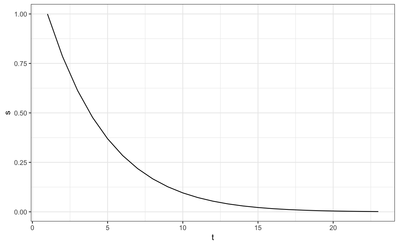 You don’t have to, but this wraps the estimated survival curve
 psi_moss_hazard_1 nicely with its corresponding time.
simultaneous confidence band (compute_simultaneous_ci)
use the following script to compute the standard error for each t on the survival curve.
survival_curve_estimate <- as.vector(moss_hazard_fit_1$survival)
eic_fit <- eic$new(
  A = df$A,
  T_tilde = df$T.tilde,
  Delta = df$Delta,density_failure = moss_hazard_fit$density_failure,
  density_censor = moss_hazard_fit$density_censor,
  g1W = moss_hazard_fit$g1W,
  psi = survival_curve_estimate,
  A_intervene = 1
)

eic_matrix <- eic_fit$all_t(k_grid = k_grid)
std_err <- compute_simultaneous_ci(eic_matrix)
upper_bound <- survival_curve_estimate + 1.96 * std_err
lower_bound <- survival_curve_estimate - 1.96 * std_err

print(survival_curve_estimate)
## [1] 1.000000000 0.785475002 0.613599337 0.477099908 0.369306980
## [6] 0.284576535 0.218293402 0.166668613 0.126663858 0.095784279
## [11] 0.072068945 0.053933388 0.040130559 0.029687804 0.021829630
## [16] 0.015948423 0.011569612 0.008335452 0.005956937 0.004215754
## [21] 0.002943700 0.002015524 0.001338971## [1] 1.4221353 1.2189637 1.0496080 0.9046808 0.7875546 0.7002686 0.6086275
## [8] 0.5500182 0.4810710 0.4507378 0.4295458 0.3879638 0.3781716 0.3729781
## [15] 0.3713365 0.2763051 0.2665923 0.2424324 0.2361423 0.2315314 0.2284484
## [22] 0.2269070 0.0366407## [1] 0.57786472 0.35198629 0.17759072 0.04951897 -0.04894061
## [6] -0.13111558 -0.17204071 -0.21668099 -0.22774326 -0.25916926
## [11] -0.28540789 -0.28009705 -0.29791047 -0.31360248 -0.32767724
## [16] -0.24440824 -0.24345306 -0.22576146 -0.22422842 -0.22309992
## [21] -0.22256101 -0.22287596 -0.03396276Session Information
## R version 3.5.3 (2019-03-11)
## Platform: x86_64-apple-darwin15.6.0 (64-bit)
## Running under: macOS Mojave 10.14.4
##
## Matrix products: default
## BLAS: /Library/Frameworks/R.framework/Versions/3.5/Resources/lib/libRblas.0.dylib
## LAPACK: /Library/Frameworks/R.framework/Versions/3.5/Resources/lib/libRlapack.dylib
##
## locale:
## [1] en_US.UTF-8/en_US.UTF-8/en_US.UTF-8/C/en_US.UTF-8/en_US.UTF-8
##
## attached base packages:
## [1] stats     graphics  grDevices utils     datasets  methods   base
##
## other attached packages:
## [1] ggplot2_3.1.1       MOSS_1.1.2          R6_2.4.0
## [4] survtmle_1.1.1      SuperLearner_2.0-24 nnls_1.4
## [7] simcausal_0.5.5
##
## loaded via a namespace (and not attached):
##  [1] Rcpp_1.0.1        plyr_1.8.4        compiler_3.5.3
##  [4] pillar_1.3.1      iterators_1.0.10  tools_3.5.3
##  [7] digest_0.6.18     gtable_0.3.0      evaluate_0.13
## [10] memoise_1.1.0     tibble_2.1.1      lattice_0.20-38
## [13] pkgconfig_2.0.2   rlang_0.3.4       foreach_1.4.4
## [16] Matrix_1.2-17     igraph_1.2.4      ggsci_2.9
## [19] commonmark_1.7    yaml_2.2.0        speedglm_0.3-2
## [22] pkgdown_1.3.0     xfun_0.6          withr_2.1.2
## [25] stringr_1.4.0     dplyr_0.8.0.1     roxygen2_6.1.1
## [28] xml2_1.2.0        knitr_1.22        desc_1.2.0
## [31] fs_1.2.7          glmnet_2.0-16     rprojroot_1.3-2
## [34] grid_3.5.3        tidyselect_0.2.5  glue_1.3.1
## [37] data.table_1.12.2 rmarkdown_1.12    tidyr_0.8.3
## [40] purrr_0.3.2       magrittr_1.5      codetools_0.2-16
## [43] scales_1.0.0      backports_1.1.4   htmltools_0.3.6
## [46] MASS_7.3-51.4     assertthat_0.2.1  colorspace_1.4-1
## [49] labeling_0.3      stringi_1.4.3     lazyeval_0.2.2
## [52] munsell_0.5.0     crayon_1.3.4